The confusion matrix is a tool to summarize prediction results of a classifier. It displays correct and incorrect prediction counts for each target class.
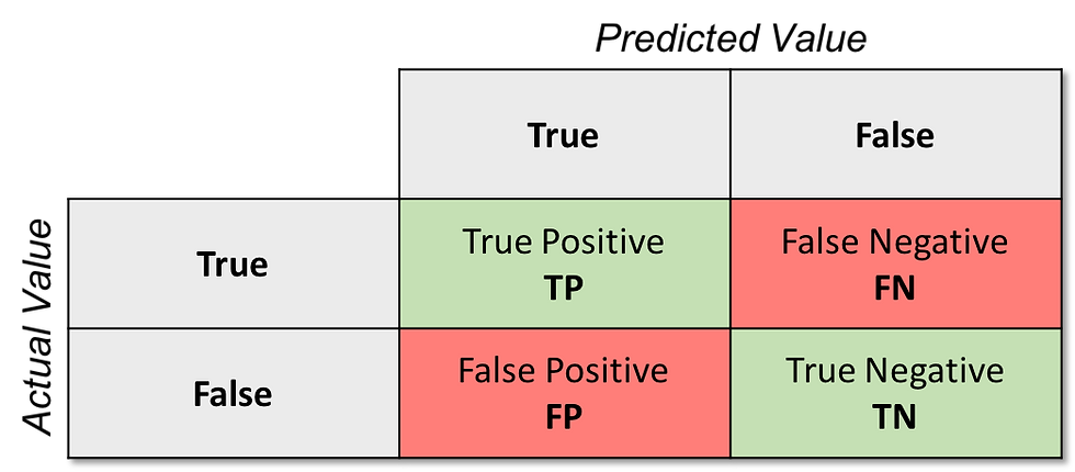
In its basic form, i.e., a binary clasification case, the confusion matrix is a two by two matrix, where rows and columns correspond to actual and predicted values, respectively. Outputs of a classifier can be labeled as True Positive (TP), False Positive (FP), True Negative (TN), and False Negative (FN).
TP represents the number of correctly classified positive samples.
FP represents the number of negative samples incorrectly classified as positive. FP is also known as Type-I error.
TN represents the number of correctly classified negative samples.
FN represents the number of positive samples incorrectly classified as negative. FN is also known as Type-II error.

Let us have a concrete example and assume a binary classifier to label patients as has breast cancer (True) or not (False).
TP represents the number of cancer patients correctly classified.
FP represents the number of not cancer patients incorrectly classified as having cancer.
TN represents the number of not cancer patients correctly classified.
FN represents the number of cancer patients incorrectly classified as having no cancer.
We will use the Breast Cancer Wisconsin (Diagnostic) Data Set publicly available on the UCI Machine Learning Repository.
Assume the data has been retrieved and transformed (i.e., missing values handled, data is scaled, and split into train and test sets) into a format ready to build a machine learning (ML) model. At this point, one can easily build an ML model:
# We will build a Logistic Regression model
# We have randomly picked this algorithm and its parameters
lr = LogisticRegression(random_state = seed, solver = 'lbfgs')
lr.fit(X_train, y_train)

# Print model's accuracy on the training data.
print('Logistic Regression Training Accuracy:',
                              lr.score(X_train, y_train))
Logistic Regression Training Accuracy: 0.9671361502347418We randomly picked the Logistic Regression algorithm to build a model. It seems the algorithm does well on the training data.
Let us see how it works on the test data, i.e., the unseen data. Before that, we need to determine the metrics we are interested in.
Accuracy of an algorithm is represented as the ratio of correctly classified patients (TP+TN) to the total number of patients (TP+TN+FP+FN).
Accuracy = (TP+TN) / (TP+TN+FP+FN)
Precision of an algorithm is represented as the ratio of correctly classified patients with the disease (TP) to the total patients predicted to have the disease (TP+FP).
Precision = TP / (TP+FP)
Recall metric is defined as the ratio of correctly classified diseased patients (TP) divided by total number of patients who have actually the disease. The perception behind recall is how many patients have been classified as having the disease. Recall is also called as sensitivity.
Recall = TP / (TP+FN)
F1 score is also known as the F Measure. The F1 score states the equilibrium between the precision and the recall.
F1Score = (2*Precision*Recall) / (Precision+Recall)
Now, we are ready to evaluate our ML model. We will simply make predictions by using the test data and compare the results with the actual values.
# Let's see how our model behaves with unseen data
# Make predictions by using the test data
y_hat = lr.predict(X_test)

# Compute the confusion matrix
cm = confusion_matrix(y_test, y_hat)

TN = cm[0][0]
FP = cm[0][1]
FN = cm[1][0]
TP = cm[1][1]

print("Confusion Matrix\n", cm, "\n")

# We can use an available method to compute accuracy
print('Testing Accuracy = ', accuracy_score(y_test, y_hat))

# Check precision, recall, f1-score in a detailed report
print("\nClassification Report:")
print("----------------------\n")
print(classification_report(y_test, y_hat))
Confusion Matrix
 [[90  0]
 [ 3 50]]

Testing Accuracy =  0.9790209790209791

Classification Report:
----------------------

              precision    recall  f1-score   support

           0       0.97      1.00      0.98        90
           1       1.00      0.94      0.97        53

    accuracy                           0.98       143
   macro avg       0.98      0.97      0.98       143
weighted avg       0.98      0.98      0.98       143
The model performs well on the test data, too. That is, 0.979, 1.00, 0.94, and 0.97 for accuracy, precision, recall, and f1-score.
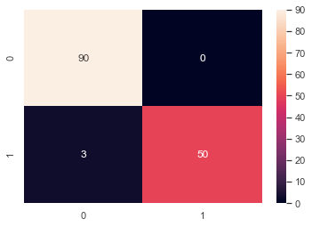
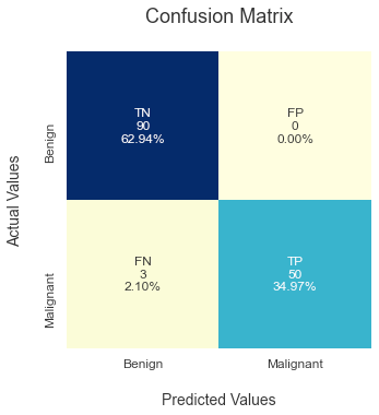
We can further visualize the confusion matrix for better understanding as well as better presentation. Remember, visualization is a preferred way of communicating when it comes to data science. A picture is worth a thousand words.
We will use a heat map to visualize the confusion matrix. I suggest you start drawing your confusion matrix in a minimal form as below.
sns.heatmap(cm, annot=True)
Then, you can easily customize your confusion matrix as you desire.
# Visualize the confusion matrix
sns.set(color_codes=True)
plt.figure(1, figsize=(5, 5))
classes = ["Benign", "Malignant"]

group_names = ['TN','FP','FN','TP']
group_counts = ["{0:0.0f}".format(value) for value in cm.flatten()]
group_percentages = ["{0:.2%}".format(value) for value in cm.flatten()/np.sum(cm)]

labels = [f"{v1}\n{v2}\n{v3}" for v1, v2, v3 in zip(group_names, group_counts, group_percentages)]
labels = np.asarray(labels).reshape(2,2)

ax = sns.heatmap(cm, annot=labels, fmt='',
                                cmap="YlGnBu", cbar=False)
ax.set_title('Confusion Matrix\n', size=18);
ax.set_xlabel('\nPredicted Values', size=14)
ax.set_ylabel('Actual Values\n', size=14);
ax.xaxis.set_ticklabels(classes, size = 12)
ax.yaxis.set_ticklabels(classes, size = 12)
And finally, let us compute some metrics manually and see if we can obtain the same values presented in the classification report.
# Finally, compute some metrics manually to see if everything checks out
Accuracy = (TP + TN) / (TP + TN + FN + FP)
Recall = TP / (TP + FN)
Precision = TP / (TP + FP)
F1Score = 2 * Precision * Recall / (Precision + Recall)

print("Accuracy = (TP + TN) / (TP + TN + FN + FP) = ", Accuracy)
print("Recall = TP / (TP + FN) = ", Recall)
print("Precision = TP / (TP + FP) = ", Precision)
print("F1-score = 2 * Precision * Recall /
                                (Precision + Recall) = ", F1Score)
Accuracy = (TP + TN) / (TP + TN + FN + FP) = 0.9790209790209791
Recall = TP / (TP + FN) = 0.9433962264150944
Precision = TP / (TP + FP) = 1.0
F1-score = 2 * Precision * Recall /
(Precision + Recall) = 0.970873786407767Yes, it works! We obtained 0.979, 1.00, 0.94, and 0.97 for accuracy, precision, recall, and f1-score again :-)
Thank you for reading this post. If you have anything to say/object/correct, please drop a comment down below.
The code used in this post is available at GitHub. Feel free to use, distribute, or contribute.

Comments